groundwater2D tutorials
The 2D groundwater solvers are designed to simulate steady and transient groundwater flows in porous media. These solvers use the Dupuit-Forchheimer approximation to simplify the modeling of flow by neglecting the vertical velocity component, which reduces the problem to two dimensions. This is ideal for large-scale simulations of aquifers or watersheds.
The examples provided in the directory tutorials/groundwater2DFoam-tutorials/ illustrate the usage of the groundwater2DFoam solver.
Steady-State Validation: steadyGroundwater2DFoam
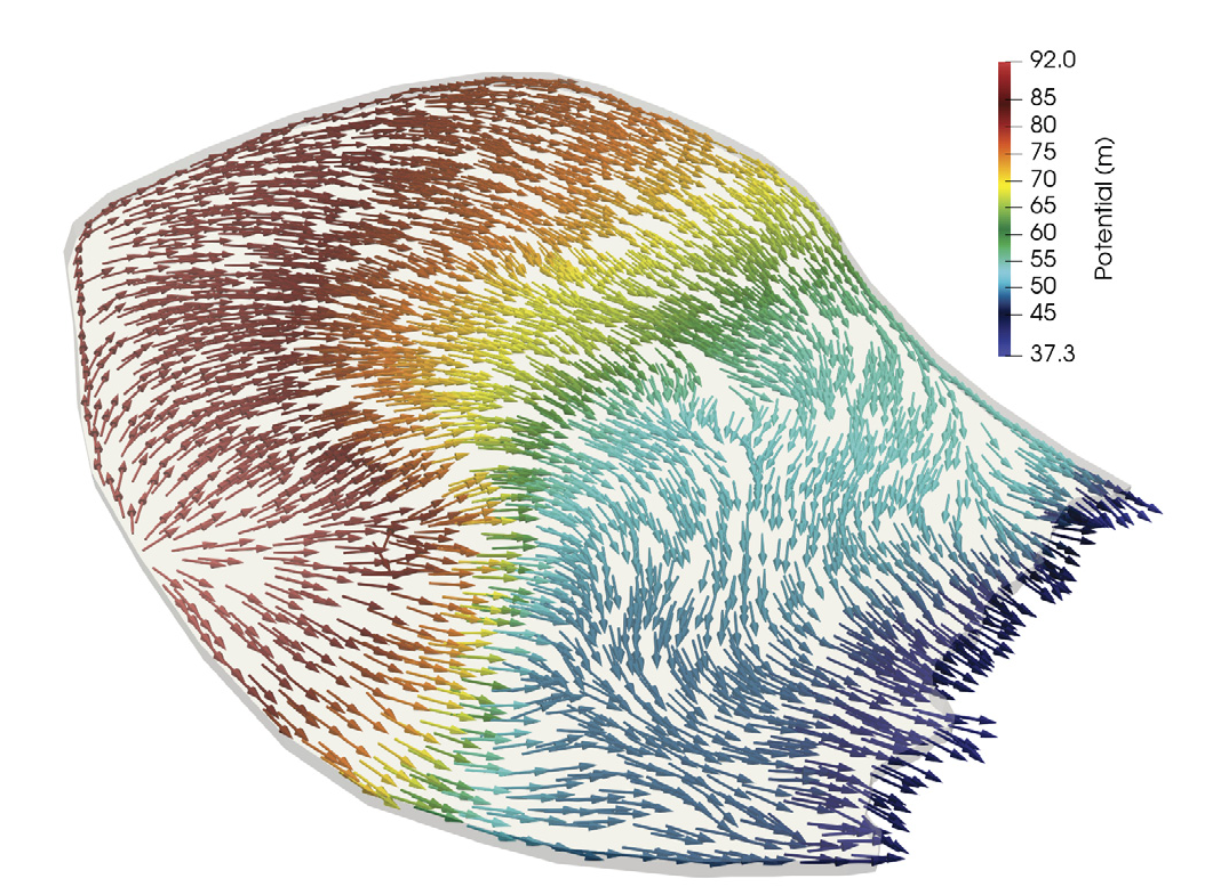
This case simulates a steady-state groundwater flow in a 2D watershed with a homogeneous infiltration rate. The configuration is set with an infiltration velocity of \(V_{infiltration} = 5.59 \times 10^{-9} \text{ m}. \text{s}^{-1}\). The boundary conditions include a Dirichlet condition at the outlet and Neumann conditions on the watershed boundaries.
The solver computes the distribution of water potential and velocity across the watershed until a steady state is reached. The results are presented below, showing the groundwater potential (water head) distribution and the corresponding velocity field and the comparison of the simulated water head values with the reference solution at selected probes confirms the solver’s accuracy:
|

|
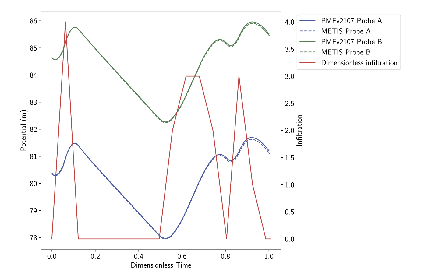
Transient Validation: groundwater2DFoam
This case starts from the steady-state configuration described above. The infiltration rate is made time-dependent, fluctuating between 0 and 4 times the reference value of \(V_{infiltration} = 5.59 \times 10^{-9} \text{ m}. \text{s}^{-1}\) over a period of 4861 days. This setup simulates the dynamic behavior of groundwater flow in response to changing infiltration conditions.
The evolution of water potential at two selected probes (A and B) over time shows a good agreement with the reference solution, validating the transient behavior of the solver: